Model Design

Governing Equation Set

\[\begin{split}\begin{align} \frac{\partial \zeta}{\partial t} &= -\left(\frac{\partial (u\zeta)}{\partial x} + \frac{1}{\overline{\rho}}\frac{\partial (\overline{\rho} w\zeta)}{\partial z}\right) + \frac{g}{\rho_0} \frac{\partial (\frac{\theta_v'}{\overline{\theta_v}} - q_c - q_r)}{\partial x} + K_x \frac{\partial ^2 \zeta}{\partial x^2} + K_z\frac{\partial ^2 \zeta}{\partial z^2} \tag{1}\\ \frac{\partial \theta}{\partial t} &= -\left(\frac{\partial u\theta}{\partial x} + \frac{1}{\overline{\rho}}\frac{\partial \overline{\rho} w\theta}{\partial z}\right) + \frac{L_v}{C_p \overline{\pi}}(C-E) + K_x \frac{\partial ^2 \theta}{\partial x^2} + K_z\frac{\partial ^2 \theta}{\partial z^2} \tag{2}\\ \frac{\partial q_v}{\partial t} &= -\frac{\partial uq_v}{\partial x} - \frac{1}{\overline{\rho}}\frac{\partial \overline{\rho}wq_v}{\partial z} - C + E + K_x\frac{\partial^{2} q_v}{\partial x^{2}} + K_z\frac{\partial^{2} q_v}{\partial z^{2}} \tag{3}\\ \frac{\partial q_c}{\partial t} &= -\frac{\partial uq_c}{\partial x} - \frac{1}{\overline{\rho}}\frac{\partial \overline{\rho}wq_c}{\partial z} + C - A - B +K_x\frac{\partial^{2} q_c}{\partial x^{2}} + K_z\frac{\partial^{2} q_c}{\partial z^{2}} \tag{4}\\ \frac{\partial q_r}{\partial t} &= -\frac{\partial uq_r}{\partial x} - \frac{1}{\overline{\rho}}\frac{\partial \overline{\rho}(w - \vec{V_T})q_r}{\partial z} + A + B - E + K_x\frac{\partial^{2} q_r}{\partial x^{2}} + K_z\frac{\partial^{2} q_r}{\partial z^{2}} \tag{5}\\ \bar{\rho}\frac{\partial \zeta}{\partial x} &= \frac{\partial^2 w}{\partial x^{2}} + \frac{\partial}{\partial z}\left(\frac{1}{\overline{\rho}}\frac{\partial (\overline{\rho}w)}{\partial z}\right) \tag{6}\\ u_{top} &= u_{\chi} + \bar{u}^{xy}, u_x = \frac{\partial \chi}{\partial x} \tag{7}\\ \frac{\partial^2 \chi}{\partial x^2} &= -\frac{1}{\bar{\rho}}\frac{\partial \bar{\rho} w}{\partial z} \tag{8}\\ \frac{\partial \bar{u}^{xy}}{\partial t} &= -\frac{1}{\overline{\rho}}\frac{\partial (\overline{\rho}\ \overline{uw}^{xy})}{\partial z} \tag{9}\\ u &= \int_{z_{top}}^{z_{bottom}} (\frac{\partial w}{\partial x} - \overline{\rho}\zeta)dz + u_{top} \tag{10}\\ \end{align}\end{split}\]

How this model works

1. Predict \(\zeta,\ \theta,\ q_v,\ q_c,\ q_r\)

2. Solving 2D poisson equation to get \(w\). The detailed process will be shown below.

3. Solving 1D poisson equation for \(\chi\) and integrate from model top to get \(u\) in the domain.

4. Iterate to the next step

Grid Setting

Boundary Condition

• Periodic boundary condition is adopted in x-direction.

• Rigid boundary condition is given in z-direction.

• The boundary condition for \(\zeta,\ \theta,\ q_v,\ q_c,\ q_r\) are given as below:

  • For x-direction:

    \[\begin{split}\begin{aligned} \zeta_{i,0} &= \zeta_{i,nz-1};\ \zeta_{i,nz-1} = \zeta_{i,1}\\ w_{i,0} &= w_{i,nz-1};\ w_{i,nz-1} = w_{i,1}\\ u_{i,0} &= u_{i,nz-1};\ u_{i,nz-1} = u_{i,1}\\ \theta_{i,0} &= \theta_{i,nz-1};\ \theta_{i,nz-1} = \theta_{i,1}\\ q_{v,i,0} &= q_{v,i,nz-1};\ q_{v,i,nz-1} = q_{v,i,1}\\ q_{c,i,0} &= q_{c,i,nz-1};\ q_{c,i,nz-1} = q_{c,i,1}\\ q_{r,i,0} &= q_{r,i,nz-1};\ q_{r,i,nz-1} = q_{r,i,1}\\ \end{aligned}\end{split}\]

  • For z-direction:

    \[\begin{split}\begin{aligned} \zeta_{i,0} &= \zeta_{i,1} = \zeta_{i,nz-1} = 0\\ w_{i,0} &= w_{i,1} = w_{i,nz-1} = 0\\ u_{i,0} &= u_{i,1}, u_{i,nz-1} = u_{i,nz-2}\\ \theta_{i,0} &= \theta_{i,1}, \theta_{i,nz-1} = \theta_{i,nz-2}\\ q_{v,i,0} &= q_{v,i,1}, q_{v,i,nz-1} = q_{v,i,nz-2}\\ q_{c,i,0} &= q_{c,i,1}, q_{c,i,nz-1} = q_{c,i,nz-2}\\ q_{r,i,0} &= q_{r,i,1}, q_{r,i,nz-1} = q_{r,i,nz-2}\\ \end{aligned}\end{split}\]

Discretization of the Governing Equation Set

Advection for Thermo-related Variables

Here presents the discretization for variables such as \(\theta,\ q_v,\ q_c,\ q_r\).

\[\frac{\partial q}{\partial t} = -\frac{\partial uq_v}{\partial x} - \frac{1}{\overline{\rho}}\frac{\partial \overline{\rho}wq_v}{\partial z} = -\frac{1}{dx} (F_r - F_l) - \frac{1}{dz} (F_u - F_d) \tag{11}\]

\[\begin{split}F_r &= u_{i+1,k}(q_{i+1,k} - q_{i,k}),\ F_l = u_{i,k}(q_{i,k} - q_{i-1,k})\\ F_u &= w_{i,k+1}(q_{i,k+1} - q_{i,k}),\ F_d = w_{i,k}(q_{i,k} - q_{i,k-1})\end{split}\]

Advection for Vorticity

The reason why we need to process the advection for vorticity seperately is due to the conservation of enstrophy. According to Arakawa (1966), the enstrophy needs to be conserved to do the long-term integration. Here, the J6 Arakawa jacobian is adopted to conserve the enstrophy following the techinical report in Jung (2005) for 3DVVM.

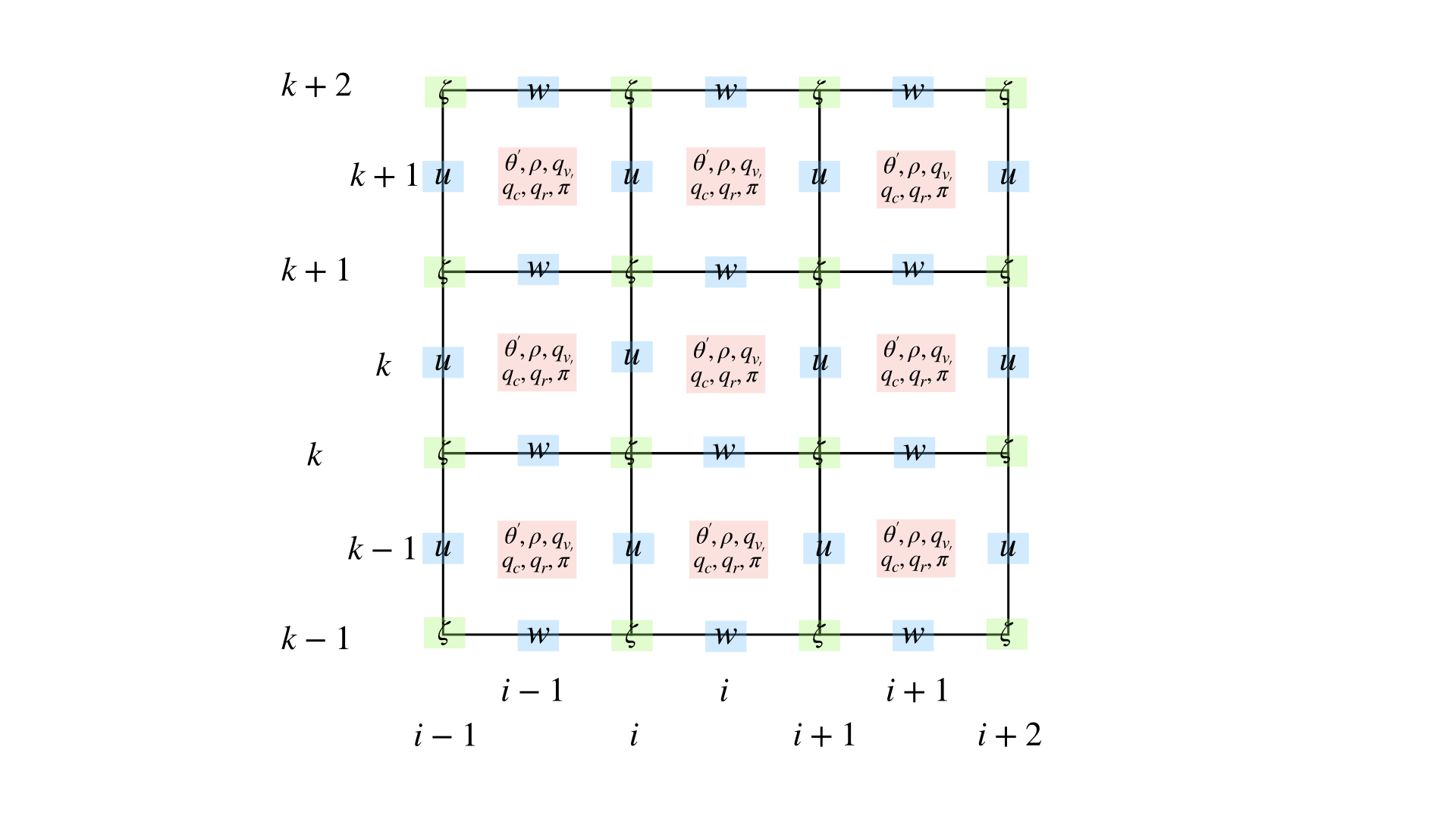
\[\frac{\partial \zeta}{\partial t} = -\frac{\partial u\zeta}{\partial x} - \frac{1}{\overline{\rho}}\frac{\partial \overline{\rho}w\zeta}{\partial z} = -\frac{1}{dx} (F_r - F_l) - \frac{1}{dz} (F_u - F_d) \tag{12}\]

\[\begin{split}F_r &= U_{i,k}(\zeta_{i+1,k} - \zeta_{i,k}),\ F_l = U_{i-1,k}(\zeta_{i,k} - \zeta_{i-1,k})\\ F_u &= W_{i,k}(\zeta_{i,k+1} - \zeta_{i,k}),\ F_d = W_{i,k-1}(\zeta_{i,k} - \zeta_{i,k-1})\\ U_{i,k} &= 0.25 \times (\overline{\rho}_k(u_{i+1,k} + u_{i,k}) + \overline{\rho}_{k-1}(u_{i+1,k-1} + u_{u,k-1}) )\end{split}\]

Solving 2D Poisson equation to diagnize \(w\)

\[\begin{split}\bar{\rho}\frac{\partial \zeta}{\partial x} &= \frac{\partial^2 w}{\partial x^{2}} + \frac{\partial}{\partial z}\left(\frac{1}{\overline{\rho}}\frac{\partial (\overline{\rho}w)}{\partial z}\right)\\ \Rightarrow \overline{\rho}^2\frac{\partial \zeta}{\partial x} &= \frac{\partial^2 \bar{\rho}w}{\partial x^{2}} + \bar{\rho}\frac{\partial}{\partial z}\left(\frac{1}{\overline{\rho}}\frac{\partial (\overline{\rho}w)}{\partial z}\right)\\\end{split}\]

\[\begin{split}\frac{\overline{\rho_{w,k}}^2}{dx}(\zeta_{i+1,k}-\zeta_{i,k}) = &\frac{1}{dx^2}(\overline{\rho_{w,k}}w_{i+1,k} - 2\overline{\rho_{w,k}}w_{i,k} + \overline{\rho_{w,k}}w_{i-1,k})\\ + &\frac{1}{dz^2}(\frac{\overline{\rho_{w,k}}}{\overline{\rho_{u,k}}}\overline{\rho_{w,k}}w_{i,k+1} - (\frac{\overline{\rho_{w,k}}}{\overline{\rho_{u,k}}} + \frac{\overline{\rho_{w,k}}}{\overline{\rho_{u,k-1}}}) \overline{\rho_{w,k}}w_{i,k} + \frac{\overline{\rho_{w,k}}}{\overline{\rho_{u,k-1}}}\overline{\rho_{w,k-1}}w_{i,k-1} )\end{split}\]

• The discretization form can be written into matrix form \(A\vec{w} = \vec{b}\).

• First, the boundary condition should be given. The periodic boundary is adopted in x-direction and the rigid boundary condition is given in z-direction.

• Assume there are n grids in x-direction, m grids in z-direction.

  • For x-direction: \(w_{0,k} = w_{nz-2,k},\ w_{nz-1,k} = w_{1,k}\).

  • For z-direction: \(w_{i,0} = w_{i,nz-1} = 0\) are boundaries, and \(w_{i,1} = 0\) is physical ground and prescribed to be 0.

• The dimension of A would be \(((nx-2)(nz-3),\ (nx-2)(nz-3))\), and \(\vec{w},\ \vec{b}\) would be ((nx-2)*(nz-3)).

  • The size of matrix D, E, and F would be \((nx-2, nz-3)\).

• In this model, dx = dz. The matrix A can be written as below:

\[\begin{split}\begin{equation*} A = \begin{bmatrix} ~D & E & ~0 & ~0 & ~0 & \ldots & ~0 \\ F & ~D & E & ~0 & ~0 & \ldots & ~0 \\ ~0 & F & ~D & E & ~0 & \ldots & ~0 \\ \vdots & \ddots & \ddots & \ddots & \ddots & \ddots & \vdots \\ ~0 & \ldots & ~0 & F & ~D & E & ~0 \\ ~0 & \ldots & \ldots & ~0 & F & ~D & E \\ ~0 & \ldots & \ldots & \ldots & ~0 & F & ~D \end{bmatrix} \end{equation*}\end{split}\]

\[\begin{split}\begin{equation*} D = \begin{bmatrix} -2-(\frac{\overline{\rho_{w,k}}}{\overline{\rho_{u,k}}} + \frac{\overline{\rho_{w,k}}}{\overline{\rho_{u,k-1}}}) & 1 & ~0 & ~0 & ~0 & \ldots & ~1 \\ 1 & -2- (\frac{\overline{\rho_{w,k}}}{\overline{\rho_{u,k}}} + \frac{\overline{\rho_{w,k}}}{\overline{\rho_{u,k-1}}})& 1 & ~0 & ~0 & \ldots & ~0 \\ ~0 & 1 & -2- (\frac{\overline{\rho_{w,k}}}{\overline{\rho_{u,k}}} + \frac{\overline{\rho_{w,k}}}{\overline{\rho_{u,k-1}}})& 1 & ~0 & \ldots & ~0 \\ \vdots & \ddots & \ddots & \ddots & \ddots & \ddots & \vdots \\ ~0 & \ldots & ~0 & 1 & -2- (\frac{\overline{\rho_{w,k}}}{\overline{\rho_{u,k}}} + \frac{\overline{\rho_{w,k}}}{\overline{\rho_{u,k-1}}}) & 1 & ~0 \\ ~0 & \ldots & \ldots & ~0 & 1 & -2- (\frac{\overline{\rho_{w,k}}}{\overline{\rho_{u,k}}} + \frac{\overline{\rho_{w,k}}}{\overline{\rho_{u,k-1}}}) & 1 \\ ~1 & \ldots & \ldots & \ldots & ~0 & 1 & -2-(\frac{\overline{\rho_{w,k}}}{\overline{\rho_{u,k}}} + \frac{\overline{\rho_{w,k}}}{\overline{\rho_{u,k-1}}}) \end{bmatrix} \end{equation*}\end{split}\]

\[\begin{split}\begin{equation*} E = \begin{bmatrix} ~\frac{\overline{\rho_{w,k}}}{\overline{\rho_{u,k}}} & 0 & ~0 & ~0 & ~0 & \ldots & ~0 \\ 0 & ~\frac{\overline{\rho_{w,k}}}{\overline{\rho_{u,k}}} & 0 & ~0 & ~0 & \ldots & ~0 \\ ~0 & 0 & ~\frac{\overline{\rho_{w,k}}}{\overline{\rho_{u,k}}} & 0 & ~0 & \ldots & ~0 \\ \vdots & \ddots & \ddots & \ddots & \ddots & \ddots & \vdots \\ ~0 & \ldots & ~0 & 0 & ~\frac{\overline{\rho_{w,k}}}{\overline{\rho_{u,k}}} & 0 & ~0 \\ ~0 & \ldots & \ldots & ~0 & 0 & ~\frac{\overline{\rho_{w,k}}}{\overline{\rho_{u,k}}} & 0 \\ ~0 & \ldots & \ldots & \ldots & ~0 & 0 & ~\frac{\overline{\rho_{w,k}}}{\overline{\rho_{u,k}}} \end{bmatrix} \end{equation*}\end{split}\]

\[\begin{split}\begin{equation*} F = \begin{bmatrix} ~\frac{\overline{\rho_{w,k}}}{\overline{\rho_{u,k-1}}} & 0 & ~0 & ~0 & ~0 & \ldots & ~0 \\ 0 & ~\frac{\overline{\rho_{w,k}}}{\overline{\rho_{u,k-1}}} & 0 & ~0 & ~0 & \ldots & ~0 \\ ~0 & 0 & ~\frac{\overline{\rho_{w,k}}}{\overline{\rho_{u,k-1}}} & 0 & ~0 & \ldots & ~0 \\ \vdots & \ddots & \ddots & \ddots & \ddots & \ddots & \vdots \\ ~0 & \ldots & ~0 & 0 & ~\frac{\overline{\rho_{w,k}}}{\overline{\rho_{u,k-1}}} & 0 & ~0 \\ ~0 & \ldots & \ldots & ~0 & 0 & ~\frac{\overline{\rho_{w,k}}}{\overline{\rho_{u,k-1}}} & 0 \\ ~0 & \ldots & \ldots & \ldots & ~0 & 0 & ~\frac{\overline{\rho_{w,k}}}{\overline{\rho_{u,k-1}}} \end{bmatrix} \end{equation*}\end{split}\]

\[\begin{split}\vec{w} = \begin{bmatrix} w_{1,2} \\ w_{2,2} \\ \vdots \\ w_{nx-2,2} \\ w_{1,3} \\ w_{2,3} \\ \vdots \\ w_{nx-2,3} \\ \vdots \\ w_{1,nz-2} \\ w_{2,nz-2} \\ \vdots \\ w_{nx-2,nz-2} \\ \end{bmatrix}\end{split}\]

\[\begin{split}\vec{b} = dx\begin{bmatrix} \overline{\rho_{w,2}}^2(\zeta_{2,2}-\zeta_{1,2}) \\ \overline{\rho_{w,2}}^2(\zeta_{3,2}-\zeta_{2,2}) \\ \vdots \\ \overline{\rho_{w,2}}^2(\zeta_{nx-2,2}-\zeta_{nx-3,2}) \\ \overline{\rho_{w,3}}^2(\zeta_{2,3}-\zeta_{1,3}) \\ \overline{\rho_{w,3}}^2(\zeta_{3,3}-\zeta_{2,3}) \\ \vdots \\ \overline{\rho_{w,3}}^2(\zeta_{nx-2,3}-\zeta_{nx-3,3}) \\ \vdots \\ \overline{\rho_{w,nz-2}}^2(\zeta_{2,nz-2}-\zeta_{1,nz-2}) \\ \overline{\rho_{w,nz-2}}^2(\zeta_{3,nz-2}-\zeta_{2,nz-2}) \\ \vdots \\ \overline{\rho_{w,nz-2}}^2(\zeta_{nx-2,nz-2}-\zeta_{nx-3,nz-2}) \\ \end{bmatrix}\end{split}\]

Solving 1D Poisson equation to diagonize \(u\)

\[\frac{\partial^2 \chi}{\partial x^2} = -\frac{1}{\bar{\rho}}\frac{\partial \bar{\rho} w}{\partial z}\]

\[\frac{1}{dx^2}(\chi_{i+1,nz-2}-2\chi_{i,nz-2}+\chi_{i,nz-2}) = -\frac{1}{dz}(\frac{1}{\overline{\rho_{u,nz-2}}}(0 - \overline{\rho_{w,nz-2}} w_{i,nz-2}))\]

• The discretization form can be written into matrix form \(G\vec{\chi} = \vec{h}\).

\[\begin{split}\begin{equation*} G = \begin{bmatrix} ~-2 & 1 & ~0 & ~0 & ~0 & \ldots & ~1 \\ 1 & ~-2 & 1 & ~0 & ~0 & \ldots & ~0 \\ ~0 & 1 & ~-2 & 1 & ~0 & \ldots & ~0 \\ \vdots & \ddots & \ddots & \ddots & \ddots & \ddots & \vdots \\ ~0 & \ldots & ~0 & 1 & ~-2 & 1 & ~0 \\ ~0 & \ldots & \ldots & ~0 & 1 & ~-2 & 1 \\ ~1 & \ldots & \ldots & \ldots & ~0 & 1 & ~-2 \end{bmatrix} \end{equation*}\end{split}\]

\[\begin{split}\vec{\chi} = \begin{bmatrix} \chi_{1,nz-2} \\ \chi_{2,nz-2} \\ \vdots \\ \chi_{nx-2,nz-2} \\ \end{bmatrix}\end{split}\]

\[\begin{split}\vec{h} = dx\begin{bmatrix} \frac{1}{\overline{\rho_{u,nz-2}}}\overline{\rho_{w,nz-2}}w_{1,nz-2} \\ \frac{1}{\overline{\rho_{u,nz-2}}}\overline{\rho_{w,nz-2}}w_{2,nz-2} \\ \vdots \\ \frac{1}{\overline{\rho_{u,nz-2}}}\overline{\rho_{w,nz-2}}w_{nx-2,nz-2} \\ \end{bmatrix}\end{split}\]